Automatic report generation

One of the things I'm working on now on the develop branch of enmtools is code to automatically generate html reports on model structure and performance.  The goal here is to provide an accessible maxent-style output with as little hassle as possible.  The current structure is just a skeleton, but I think it's already pretty neat.  Here's a sample html report for a GAM, exactly as it comes out of enmtools:

Summary of ENMTools gam object for allogus

Spatial prediction

Model: presence ~ s(layer.1, k = 4) + s(layer.2, k = 4) + s(layer.3, , k = 4) + s(layer.4, k = 4)

## 
## Family: binomial 
## Link function: logit 
## 
## Formula:
## presence ~ s(layer.1, k = 4) + s(layer.2, k = 4) + s(layer.3, 
##     k = 4) + s(layer.4, k = 4)
## 
## Parametric coefficients:
##             Estimate Std. Error z value Pr(>|z|)    
## (Intercept)  -3.3732     0.1911  -17.65   <2e-16 ***
## ---
## Signif. codes:  0 '***' 0.001 '**' 0.01 '*' 0.05 '.' 0.1 ' ' 1
## 
## Approximate significance of smooth terms:
##              edf Ref.df Chi.sq  p-value    
## s(layer.1) 1.641  1.994  1.101  0.57526    
## s(layer.2) 1.000  1.001 26.379 2.81e-07 ***
## s(layer.3) 2.850  2.963 10.804  0.00856 ** 
## s(layer.4) 2.725  2.922  8.414  0.03309 *  
## ---
## Signif. codes:  0 '***' 0.001 '**' 0.01 '*' 0.05 '.' 0.1 ' ' 1
## 
## R-sq.(adj) =  0.0661   Deviance explained = 12.7%
## UBRE = -0.63881  Scale est. = 1         n = 1052

Evaluation

Geographic space

## class          : ModelEvaluation 
## n presences    : 52 
## n absences     : 1000 
## AUC            : 0.7715385 
## cor            : 0.2319033 
## max TPR+TNR at : -2.695771

## 
## 
## Proportion of data wittheld for model testing:

## [1] 0.2

## class          : ModelEvaluation 
## n presences    : 13 
## n absences     : 1000 
## AUC            : 0.7910385 
## cor            : 0.1300592 
## max TPR+TNR at : -3.014335

Environment space

## class          : ModelEvaluation 
## n presences    : 52 
## n absences     : 10000 
## AUC            : 0.5357038 
## cor            : -0.0329415 
## max TPR+TNR at : 0.01546464

## 
## 
## Proportion of data wittheld for model testing:

## [1] 0.2

## class          : ModelEvaluation 
## n presences    : 13 
## n absences     : 10000 
## AUC            : 0.5380154 
## cor            : -0.01697503 
## max TPR+TNR at : 0.01534051

Model fit using gam.check

## 
## Method: UBRE   Optimizer: outer newton
## full convergence after 9 iterations.
## Gradient range [-4.371328e-07,2.558592e-06]
## (score -0.6388078 & scale 1).
## Hessian positive definite, eigenvalue range [4.369759e-07,0.0004284836].
## Model rank =  13 / 13 
## 
## Basis dimension (k) checking results. Low p-value (k-index<1) may
## indicate that k is too low, especially if edf is close to k'.
## 
##               k'   edf k-index p-value
## s(layer.1) 3.000 1.641   0.932    0.47
## s(layer.2) 3.000 1.000   0.927    0.36
## s(layer.3) 3.000 2.850   0.862    0.02
## s(layer.4) 3.000 2.725   0.806    0.00

Notes

## [1] "No formula was provided, so a GAM formula was built automatically"

Citations

Warren, D.L. (2016) Package ‘enmtools’. Available online at: https://github.com/danlwarren/ENMTools

Hijmans, R.J, Phillips, S., Leathwick, J. and Elith, J. (2011), Package ‘dismo’. Available online at: http://cran.r-project.org/web/packages/dismo/index.html.

The flood becomes a trickle

Just a quick update: the flood of posts is going to slow down a bit from here on out, because I've now built enough of the framework of ENMTools that I can start working on the really cool experimental stuff I've got planned.  I will put some more time into polishing up what's already available,  beefing up the help files, etc., but won't be adding new features to the final version anywhere near as quickly.
Please absolutely do let me know when you run into problems with the R version, though!  I've got a few test data sets I can use for evaluation purposes, but it's almost certain that some of you out there will run into new issues using your own data sets.  I want to figure out what those issues are and catch them as soon as possible, so that the end product is as easy to use as I can make it.

Ecospat tests!

I haven't added this to the vignette on GitHub yet (because I just literally got it working a couple of minutes ago), but I've leveraged the enmtools.species object structure to make the equivalency and similarity tests from ecospat much more accessible.

For those that aren't familiar, these tests essentially do the same sort of thing that the identity/equivalency and background/similarity tests in good ol' ENMTools do, but they do them directly in environment space with no need to build an ENM.  Basically they make kernel density estimates of your species' occurrence in environment space, the available habitat for your species in environment space, and the environment space itself.  Then they basically "correct" the density of your species for the density of available habitat and measure overlap using I and D.  Those overlaps are then tested against a null distribution from a permutation test, much like the ones in ENMTools.

I really liked the Broennimann et al. idea when I read about it, and was super excited when ecospat came out.  The interface is a bit clunky, though, and requires a lot of setup to run.  The nice thing about the enmtools.species object structure is that I can actually automate all of this setup for you, and in the end you get a really cool ecospat test with basically zero hassle!

Oh, one note, though: ecospat only works in two environmental dimensions.  Keep that in mind, because if you try to pass the enmtools.ecospat functions more or less than two dimensions they will barf and yell at you.  If, for instance, you have two enmtools.species objects with backgrounds and presence points (named ahli and allogus here) you can call the ecospat tests like this:
And you get the good stuff you're used to by now...



esp.id = enmtools.ecospat.id(ahli, allogus, env[[c("layer.1", "layer.3")]])

esp.bg.sym = enmtools.ecospat.bg(ahli, allogus, env[[c("layer.1", "layer.3")]], test.type = "symmetric")

esp.bg.asym = enmtools.ecospat.bg(ahli, allogus, env[[c("layer.1", "layer.3")]], test.type = "asymmetric")

ecospat.id test p-values:

   D    I 

0.02 0.02 

As well as this cool sucker:

This plot shows the availability and occupancy of the environment for each species.  Neat, huh?  

Noe that these scaled densities look a little weird.  That's because I left low density thresholds for ecospat at zero (th.sp and th.env options for function ecospat.grid.clim.dyn).  Those are definitely something you should mess with, otherwise you get (as I have here) situations where the most relevant habitat to the I and D metrics is in fact some of the most marginal habitat for the species.

Check out those GAMs!

As of yesterday afternoon (Australia time), ENMTools can now do GAMs as well!  That includes all of the hypothesis tests, visualization, etc. that you get with the other methods.

Just like the recent update to the enmtools.glm() function, enmtools.gam() has the ability to automatically build a function if you don't supply one. For instance if you have four layers in a stack called "env" named "layer.1", "layer.2", etc. and call enmtools.gam() thusly:

ahli.gam = enmtools.gam(ahli, env)

The function will automatically build the function:

presence ~ s(layer.1, k = 4) + s(layer.2, k = 4) + s(layer.3, k = 4) + s(layer.4, k = 4)

 As you can see above, the default value for k, the smoothing parameter, is 4.  This is not necessarily optimal, though, and it's definitely worth exploring for your specific data.  You can either supply GAM formulas manually (using the "f" argument to enmtools.gam), or you can just provide a "k" argument, e.g,

ahli.gam = enmtools.gam(ahli, env, k = 6)

Which produces

presence ~ s(layer.1, k = 6) + s(layer.2, k = 6) + s(layer.3, k = 6) + s(layer.4, k = 6)

Formula arguments or k values can also be passed to the hypothesis testing functions (identity, background, rangebreak, etc.).

Automatic formula building for enmtools.glm()

I just added a new bit of functionality to enmtools.glm.  Nothing major, but it's kinda cool and it saves a bit of time when building GLMs that are strictly an additive function of a set of environment layers.  It used to be that you'd have to pass enmtools.glm() a formula object in order to build a model, e.g.:

ahli.glm = enmtools.glm(f = pres ~ layer.1 + layer.2 + layer.3 + layer.4, species = ahli, env = env, test.prop = 0.2)

You CAN still do that, but now you no longer have to.  Now if you don't pass it a formula, it assumes that your formula takes the form:

presence ~ layer.1 + layer.2 + ...

For every layer in your environment stack.  That means you can just call it like the other enmtools modeling functions, e.g.,

ahli.glm = enmtools.glm(species = ahli, env = env, test.prop = 0.2)

And it will use all the layers in env.  If you want a strictly additive formula that just uses a subset of those layers, you can just pass a subset of them to the env argument, like this:

ahli.glm = enmtools.glm(species = ahli, env = env[[c(1,3,5)]], test.prop = 0.2)

The function will then build a model using the formula

presence ~ env[[1]] + env[[3]] + env[[5]]

And ignore all the other layers.

If you want some sort of more complicated functional response (polynomials, interactions, etc.), you'll still need to supply the formula manually.

Visualizing ENMs in environment space

Hey, wouldn't it be nice if you could look at the predictions your ENM makes in environment space?  Well now you can!*

*two-dimensional plots only, only works with enmtools.model objects, offer void in Nebraska

With a new function that I just uploaded last night, you can take any enmtools.model object and a set of environment layers, and you can visualize the response of your model to those two layers.  Cool, huh?  Check this out:

allogus.glm = enmtools.glm(pres ~ layer.1 + layer.2 + layer.3 + layer.4, allogus, env)

plot(allogus.glm)




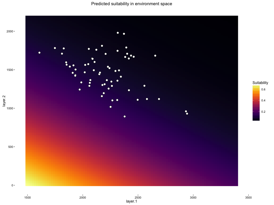
env.plots = visualize.enm(allogus.glm, env, layers = c("layer.1", "layer.2"))

env.plots

The first plot shows us the predicted suitability in environment space for two variables (layer.1 and layer.2), while holding the remaining variables constant at their mean value across all presence points.  Here's that GLM:





OH GOD THAT'S APPALLING.  It does make sense given our geographic projection of the model, though - many occurrence points have low suitability scores.  So what happened?  The second plot gives us some insight.




The colored background here shows us the relative density of our background points in environment space.  And this really points up one of the most significant conceptual things about ENMs that is worth having a good think about: presence/background methods are trying to estimate a function that distinguishes your occurrence points from your background points.  Many of the occurrences for this species are very similar to the distribution of background data.  As a result of this, these models tend to emphasize occurrences that happen in areas of environment space that are under-represented in the background.  The model is essentially being "pulled" towards those points that occur in the black/purple areas of the background density plot, and as a result it tends to extrapolate heavily into areas of environment space in the bottom left.  Where, it should be noted, we have no data of any sort.  Yikes.

Cathy Newman asked via Twitter whether there were any of these plots that don't look funky, and the answer so far is "not many"!  For Bioclim and Domain models you often get something that looks fairly reasonable, even though the geographic prediction may not be great.  For example, here's a Domain model for another species:




Doesn't look as insane in environment space as that GLM up there, but as you can see the predicted habitat suitability is not a great reflection of the species' distribution.  Which one of those models is more believable and/or useful is a very good question that I'm not going to delve into just now.  I do think these plots are really useful and interesting for thinking about the modeling process, even though what they usually tell us is that our pretty maps are often associated with shockingly weird estimates of the underlying ecology.

All of the above is in the current version of ENMTools on GitHub.  It does only work with enmtools.model objects, so you're going to need to walk through how to build those first.  There's a nice readme on the GitHub landing page that should explain a lot.




Side note: the limits of the x and y axes are set by the max and min for each layer in the environmental layers you provide.  If you want to zoom in, you can add xlim and ylim arguments after the fact.  For instance, to zoom into the first environment space plot up at the top there, we could do:

env.plots$suit.plot + xlim(c(1500,3000)) + ylim(c(900, 2100))

R users: update your R!

Hey y'all, if you're doing a bunch of SDM/ENM stuff in R and are finding that many of your operations are running really slowly, you should check your R version.  R version 3.3.0 has some sort of bug going on that causes it to handle many raster operations VERY slowly, including extracting data from a raster using points.

It's a very odd bug, because it causes the operation to get slower and slower the more points you add (which makes sense), but then suddenly gets considerably faster when you're using over 250 points.  So extracting data using 250 points might take three minutes, while 251 points takes three seconds.  Crazy, but at least the fix is easy!